A unified prediction of computer virus spread in connected networks

Lora Billings, William Spears, Ira Schwartz
Physics Letters A, 297 (2002) pp.261-266
ISSN 0375-9601
May 2002

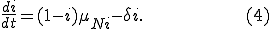
Download PDF (163.04Kb) (You need to be registered on forum)
[Back to index] [Comments (0)]

Lora Billings
Department of Mathematical Sciences, Montclair State University,
Upper Montclair, NJ 07043, USA
Corresponding author.
E-mail address: billingsl@mail.montclair.edu (L. Billings).
URL address: http://www.csam.montclair.edu/billings.

William M. Spears
Department of Computer Science, University of Wyoming,
Laramie, WY 82071, USA

Ira B. Schwartz
Naval Research Laboratory, Nonlinear Dynamics System Section, Code 6792,
Plasma Physics Division,
Washington, DC 20375, USA

Abstract

We derive two models of viral epidemiology on connected networks and compare results to simulations. The differential equation model easily predicts the expected long term behavior by defining a boundary between survival and extinction regions. The discrete Markov model captures the short term behavior dependent on initial conditions, providing extinction probabilities and the fluctuations around the expected behavior. These analysis techniques provide new insight on the persistence of computer viruses and what strategies should be devised for their control.

Concerns about our vulnerability to computer viruses have prompted a serious effort to model their spread, and to develop a detection and control mechanism that prevents widespread infection of computers connected to the internet. Because of the widespread connectivity of the internet, there has been much attention paid to the organization and transmission of information on finite networks. One such example is the small-world network [1], where a regular network is combined with a few random interconnections. Similar models have generated statistical cluster analysis based on percolation [2], scaling laws [3], and control of information [4]. Recent work on internet connectivity has shown that with the right scaling law, the internet is robust when computer attacks remove certain nodes [5]. Moreover, percolation theories have been used to model the propagation of an epidemic probabilistically [6].

Recently, traditional biological approaches have been combined with topological interconnects, such as small-world networks [1,7], percolation theory, and graph theory, to predict the conditions for which an epidemic will occur [8]. Examples are discrete algorithms based on Markov models and continuous ordinary differential equation models derived from epidemic compartmental models based on large populations [9]. In this Letter, we derive a Markov and an ordinary differential equation (ODE) model of viral epidemiology on connected networks and compare results to simulations. Using both methods, we derive a complete picture of viral propagation in a connected network.

We continue the foundation work presented by Kephart and White [10] by improving on some of their assumptions and approximations. Our Markov model is a variation of the Reed-Frost model [11] and our differential equation is a variation of the SIS model [12]. One major difference is that we do not use the assumption that only one infection can occur at a time. It is more realistic to include the probability that multiple computers can become infected (or cured) at a given instant. We have also taken a new approach to model the rate at which a node attempts to infect its neighbors. We assume that the rate depends on the number of nodes infected, not just the connectivity of a node as in [13,14]. An infection occurs in two stages. Not only is there a probability that a person can receive an infected email, but there is a probability that a person might choose not to open it. With these modifications to the model, we have improved the agreement between how the differential equation and the Markov model predict the behavior of a simulation, and derive the threshold under which a virus dies out. We exploit how the continuous model predicts the long term behavior of the system, while the discrete model captures the short term behavior dependent on initial condition. We now present these models.

To model the spread of viruses throughout a network, we assume that the network consists of nodes. Each node can be in one of two medical conditions: susceptible () or infected (). We assume discrete time steps of arbitrary units, so at any given time , S = N - I . Infected nodes can remain infected or become susceptible by being cured. Likewise, susceptible nodes can remain susceptible or become infected. Denote the probability that a susceptible node becomes infected as $\mu$ . This rate depends on two parameters, the connectivity of the network () and the probability of transmitting an infection ( $\beta$ ). The probability that an infected node becomes susceptible is $\delta$ . 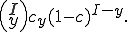Fig. 1 illustrates the transitions between these two medical conditions, with their associated probabilities.

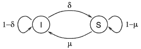
Fig. 1. The transition diagram showing how a node can change medical conditions.

A discrete-time Markov chain is a dynamical system composed of discrete states. In this Letter, the number of nodes in each medical condition will define a Markov state, forming the pair (I,S) . Because is explicitly defined by , we only refer to , and in this case, S = N + 1 . At each time step , the Markov chain can change states. We compute the probability of transitioning from state to state . Let X_n be the random variable for the Markov chain, which can take on any of the states at time . 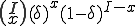The system is described by an $S \times S$ matrix , where a component of is given by

$Q(I,I') \equiv p_{I,I'} \equiv P(X_n = I' | X_{n-1} = I). \hspace{100}(1)$

Let be the number of infected nodes that are cured. Since there are infected nodes, I - x of them are not cured, and remain infected. If we use $\delta$ to denote the probability of curing an infected node, then the probability of curing of the infected nodes is

$\left(\begin{matrix}I\\x\end{matrix}\right) (\delta)^x(1 - \delta)^{I - x}$

Note that $\delta$ is a constant that reflects the strength of the immune system.

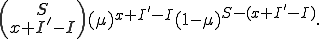
Now, since I' - I more susceptible nodes are infected than infected nodes are cured, we know that x + I' - I of the susceptible nodes must become infected. If there are susceptible nodes then 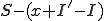S - (x + I' -I) of the susceptible nodes are not infected. Use $\mu$ to denote the probability of infecting a susceptible node. Then, the probability of infecting of the susceptible nodes is simply

$\left(\begin{matrix}S\\x + I' - I\end{matrix}\right)(\mu)^{x + I' - I}(1 - \mu)^{S - (x + I' - I)}.$

The probability that a susceptible node will become infected is largely dependent on the number of neighboring nodes in the graph that are infected, as well as the transmission probability. Therefore, $\mu$ cannot be approximated by a constant as in the case of the cure rate.

A random directed graph of nodes is constructed by making random, independent decisions about whether to include each of the N(N - 1) possible directed edges that can connect two nodes. Each edge is included in the graph with a connectivity probability . If is the total number of infected nodes, the probability of having $0 \le y \le I$ infected neighbors is

$\left(\begin{matrix}I\\y\end{matrix}\right)c_y(1 - c)^{I - y}.$

Assume that the probability that one of these infected neighbors transmits the infection is $\beta$ . If is the number of infected neighbors, then the probability that none of these neighbors will infect a given susceptible node is $(1 - \beta)^y$ . Thus the conditional probability that a given node will be infected by at least one infected neighbor is $1 - (1 - \beta)^y$ . Therefore, the probability that a susceptible node will be infected is

$\mu = \sum_{y = 0}^I\left(1 - (1 - \beta)^y\right)\left(\begin{matrix}I\\y\end{matrix}\right)c^y(1 - c)^{I - y}.\hspace{100}(2)$

Note that we do not use the approximation $\mu = {\beta}cI$ , as in [10], which approximates the correct behavior when is small, or $\beta$ and are small.

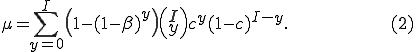
Finally, we have all the components needed to find the probability of transitioning from state to state . This is achieved by summing over all possible values of . The bounds are determined by examining the combinatorials. The first combinatorial implies that $0 \le x \le I$ . The second implies that 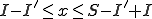$I - I' \le x \le S - I' + I$ . Satisfying all of these constraints, we get

$p_{I,I'} = \sum_{x=\mbox{max}\{0,I-I'\}}^{\mbox{min}\{I,S-I'+I\}} \left( \begin{matrix}I\\x\end{matrix} \right) (\delta)^x(1 - \delta)^{I - x} \left( \begin{matrix}S\\x + I' - I\end{matrix} \right) \times (\mu)^{x + I' - I}(1 - \mu)^{S - (x + I' - I). \hspace{100}(3)$

With the transition matrix defined, we can use the Markov model to determine various quantities of interest, such as the probability distribution of infected nodes at time , as well as the probability of extinction. The algorithm starts with an initial condition vector of length describing which state the network is in. This vector is actually a probability density function (PDF) with one in the position that corresponds to the nodes that are initially infected. The PDF at time is computed from iterating the initial condition vector by the transition matrix times. The expected number of infected nodes is the sum of each state multiplied by its associated probability from the PDF. (This calculation is equivalent to averaging the solution from a simulation over a large number of runs.)

The absorbing state of zero infected nodes at time captures the phenomena of extinction. This is the case where only a few nodes have the virus, and by chance, it does not spread fast enough to avoid extinction. From experiments, nonzero probabilities for extinction occur when less than 10% of the nodes are initially infected, and the probabilities increase as the number of infected nodes is decreased. Extinction plays an important role later when we compare the models.

Notice at this point that the model can easily be expanded to include medical conditions, assuming that the transitions between medical conditions occur in a ring [15]. Another important point is that the parameters need not be constants - they in fact can be functions that depend on the state that the process is in (as seen in the computation of $\mu$ above). This level of generality provides for nonlinear dynamics of the system, as we will see in the following discussion concerning differential equation models of viral spread.

We continue by constructing an ordinary differential equation (ODE) that models the same process from a continuous time perspective. The advantage of this approach is that we can determine the long term behavior of the system as a function of the parameters. Therefore, we do not need to solve the ODE, just perform a stability analysis of the constant solutions. Time, , is now assumed to be continuous. We now derive the process that allows the system to change state. The number of infected nodes increases by the number of susceptible nodes that get infected. That rate is captured by $\mu S$ , which is nonlinear because of the dependence of $\mu$ on as shown in (2). The number of infected nodes decreases by the number of infected nodes that are cured, $\delta I$ . The reverse holds true for how the number of susceptible nodes change.

Let i = I/N and s = S/N be the proportion of infected and susceptible nodes (respectively). Since i + s = 1 , the system can be described in one variable by the following equation:

$\frac{di}{dt} = (1 - i)\mu_{Ni} - \delta i. \hspace{100}(4)$

with $\mu_{Ni}$ defined as $\mu$ in (2), but using the next smallest integer of nodes infected.

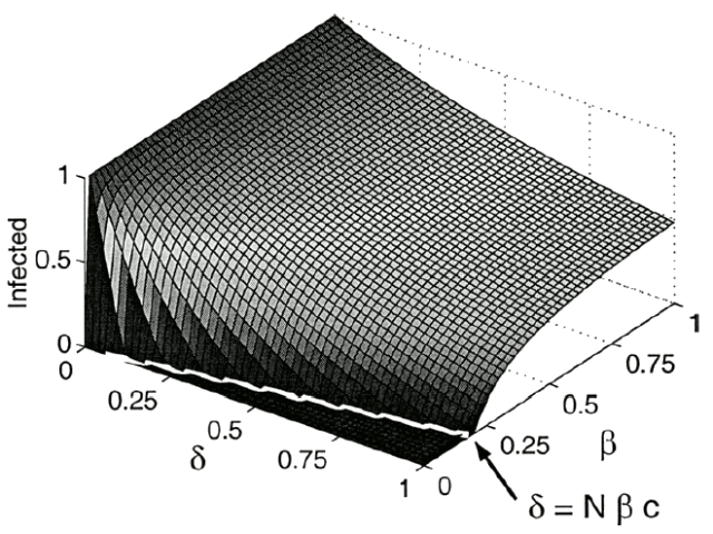
Fig. 2. The stable solution as a function of δ and β, with c = 0.0505. Note the line dividing the endemic and extinction regions, δ = Nβc.

Fig. 2. The stable solution as a function of $\delta$ and $\beta$ , with c = 0.0505. Note the line dividing the endemic and extinction regions, $\delta = N\beta{c}$ .

The constant solutions are found by solving di/dt = 0 for . The zero solution, i = 0 , exists for all $\beta$ and $\delta$ if the connectivity, $c \gt 0$ . In a region of small $\beta$ , the zero solution is stable. This region is bounded by a curve where the zero solution loses stability and a stable nonzero solution is created. This new solution is called the endemic solution, $i_e \gt 0$ . Here, the virus will not naturally die out, but persist at a constant level.

The boundary curve between the stable zero solution and the stable endemic solution is found by solving di/dt = 0 explicitly for $\delta$ and taking the limit as approaches zero from the positive side,

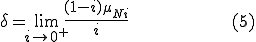
$\delta = \lim_{i \to 0^+}\frac{(1 - i)\mu_{Ni}}{i} \hspace{100}(5)$

We use the following simplification from (2):

$\frac{\mu_{Ni}}{i} = N \sum_{y = 0}^{Ni} \left(1 - (1 - \beta)^y\right) \times \frac{(Ni - 1)!}{(Ni - y)!y!} c^y (1 - c)^{Ni - y},$

and the assumption that if is small, then $\mu_{Ni} \approx \mu_1$ . Therefore, (5) can be approximated by

$\delta \approx N\beta{c}. \hspace{100}(6)$

Solutions on this line have neutral stability, slowing the convergence rates of solutions for nearby parameters. If $\delta \ge N\beta{c}$ , this model predicts that the diseasewill die out because the only solution is i = 0 . Otherwise, the disease will persist at an endemic state greater than one. See Fig. 2 for a numerical approximation of the stable solution as a function of $\beta$ and $\delta$ . Overlaid in white is the line dividing the extinction and endemic regions.

As a reality check, we also perform a simulation of the discrete system that takes nodes and tracks their status, infected or susceptible, over time. Given susceptible and infected nodes, the simulation begins by finding which susceptible nodes will become infected. For each susceptible node, an infected neighbor network is determined by a random variable coin flip (weighted by ) for each infected node. For each successful trial, another coin flip (weighted by $\beta$ ) determines if the virus is passed to the susceptible node. If the virus is passed, the process for that susceptible node is halted and condition will be changed to infected at the next time step. This process is repeated for all susceptible nodes. Next, the simulation finds which infected nodes will be cured. A random coin flip (weighted by $\delta$ ) is used for each infected node. A success results in the node changing to susceptible at the next time step. After all the nodes have been considered, instantaneously all the new conditions are updated and process is repeated. Each loop represents a time step and a run represents time steps.

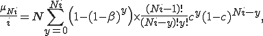
We continue with a comparison of our two models with the simulation. The expected number of connections tions emanating from a single node is c(N - 1) . We assume in a network of 100 nodes a connectivity of 5%. Therefore, in all calculations, we have fixed the connectivity parameter at c = 0.0505 . Also note that the simulation data is an average of the results over 3,000 runs. Sample time series are shown in Fig. 3.

Fig. 3. This graph shows the time series data from the Markov model and the simulation for the parameters N = 100, β = 0.1200, δ = 0.2000, and c = 0.0505. The dashed line represents the endemic state predicted by the ODE.

Fig. 3. This graph shows the time series data from the Markov model and the simulation for the parameters $N = 100, \beta = 0.1200, \delta = 0.2000$ , and . The dashed line represents the endemic state predicted by the ODE.

The Markov model and the simulation also need an initial condition in the form of the number of nodes initially infected. The initial condition is important when considering the probability of virus extinction, when the solution reaches i = 0 . In the simulation, the zero solutions are just part of the results averaged over the different trials. The Markov model captures the probability of an i = 0 solution specifically, and that is averaged in with the nonzero probabilities. As discussed in [10], the distribution splits into an "extinction" component and a "survival" component. See Fig. 4 for an example PDF. The extinction component exists only for small initial conditions. Note that the survival component has a mean of 60.2114 and a standard deviation of 5.6938. The standard deviation captures the fluctuations around the expected behavior that will happen in the separate runs of a simulation.

Table 1 shows the results for the three methods over a range of different initial conditions when $\beta = 0.1200$ and $\delta = 0.2000$ . The extinction probability from the Markov PDF is shown in the last column. After renormalizing the survival component, the nonzero solutions for both the Markov model and the simulation match the ODE prediction well. Note that the ODE can only capture the unstable i = 0 solution in the endemic region when the initial condition is i = 0 , or no nodes are infected initially.

Fig. 4. An example PDF from the Markov model. The parameters are N = 100, β = 0.1200, δ = 0.2000, c = 0.0505, and the initial condition of 1 node infected. The extinction component is at i = 0. The survival component has a mean of 60.2114 and a standard deviation of 5.6938.

Fig. 4. An example PDF from the Markov model. The parameters are $N = 100, \beta = 0.1200, \delta = 0.2000, c = 0.0505$ , and the initial condition of 1 node infected. The extinction component is at . The survival component has a mean of 60.2114 and a standard deviation of 5.6938.

Table 1. A comparison of the data for parameters $N = 100, \beta = 0.1200, \delta = 0.2000$ , and . The first column contains the initial condition used in the Markov model and the simulation. The last column shows the extinction probability found from the Markov model

I₀	ODE	Simulation	Markov	Extinction
100	60.4450	60.1575	60.2114	0
80	60.4450	60.1115	60.2114	0
60	60.4450	60.2890	60.2114	0
40	60.4450	60.1985	60.2114	0
20	60.4450	60.2050	60.2114	0
10	60.4450	60.2120	60.2111	0
8	60.4450	60.2145	60.2089	0.000004
6	60.4450	60.1705	60.1835	0.000041
4	60.4450	59.6570	59.8765	0.000462
2	60.4450	55.4790	55.8793	0.005562
1	60.4450	42.9985	44.2045	0.265845

The original results from the Markov model and the simulation tests are close for all $\beta$ and $\delta$ parameters. Renormalizing the survival component removes the dependence on initial conditions so the result matches the ODE as well. In general, the only region where the methods do not agree is near the line of neutral stability predicted by the ODE, $\delta = N\beta{c}$ . Except for extreme values of $\delta$ (near 0), even those errors are within 2%, where extremely slow convergence occurs when $\delta$ and $\beta$ are very close to zero.

The ODE model is useful for exploring how the behavior of the system varies with . Fig. 5 shows how the number of infected nodes can be reduced by simply reducing . This illustrates the effectiveness of temporarily partitioning a large network into small isolated components in order to reduce an infection. We are currently extending this framework to more diverse and nonhomogeneous networks.

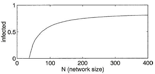
Fig. 5. This is a graph of how the long term behavior changes with the size of the network, N. For example, the parameters in the ODE are β = 0.1200, δ = 0.2000, and c = 0.0505.

Fig. 5. This is a graph of how the long term behavior changes with the size of the network, . For example, the parameters in the ODE are $\beta = 0.1200, \delta = 0.2000$ , and .

In summary, we have shown how a detailed picture of short and long term dynamics of viral propagation in connected networks can be obtained using both Markov and ODE models. We have tried to combine the traditional tools of population biology with a graph-theoretical approach of studying the persistence of computer viruses. We have focused on improving the approximation of the contact rate, which is a parameter that captures the effective transmission of a disease. By extracting the contact rate parameter from real data, we could produce a metric to predict the spread of a virus. Once a tipping point is identified, ways to control the parameter away from it could effectively prevent large-scale epidemics.

Acknowledgements

This work was supported by the Office of NavalResearch (ONR). L.B. is supported by the ONR under grant N00173-01-1-G911. We wish to thank Erik Bollt for his useful comments.

References

D. Callaway, M. Newman, S. Strogatz, D. Watts, Phys. Rev. Lett. 85 (2000) 5468.
M. Newman, D. Watts, Phys. Rev. E 60 (1999) 7332.
A. Barabasi, R. Albert, H. Jeong, Physica A 272 (1999) 173.
S. Pandit, R. Amritkar, Phys. Rev. E 60 (1999) R1119.
R. Cohen, K. Erez, D. Ben-Avraham, S. Havlin, Phys. Rev. Lett. 85 (2000) 4626.
C. Moore, M. Newman, Phys. Rev. E 61 (2000) 5678.
D. Watts, S. Strogatz, Nature 393 (1998) 440.
B. Soh, T. Dillon, P. County, Comput. Networks ISDN Syst. 27 (1995) 1447.
I. Schwartz, J. Math. Biol. 30 (1992) 473.
J. Kephart, S. White, in: Proceedings of the 1991 IEEE Computer Society Symposium on Research in Security and Privacy, 1991, pp. 343-359.
F. Hoppensteadt, Mathematical Methods of Population Biology, Cambridge University Press, Cambridge, 1982.
N. Bailey, The Mathematical Theory of Infectious Diseases and Its Applications, Oxford University Press, New York, 1975.
R. Pastor-Satorras, A. Vespignani, Phys. Rev. Lett. 86 (2001) 3200.
A.-L. Barabasi, R. Albert, H. Jeong, Physica A 281 (2000) 69.
W. Spears, L. Billings, I. Schwartz, Modeling viral epidemiology, Naval Research Laboratory, NRL/MR/6700-01-8537, 2001.

[Back to index] [Comments (0)]

VX Heavens

A unified prediction of computer virus spread in connected networks

Abstract

Acknowledgements

References