Wing Wong, Mark Stamp
Journal In Computer Virology vol. 2, no 3
ISSN 1772-9904
December 2006
 Download PDF (989.46Kb) (You need to be registered on forum)
A talk based on the results in this paper was presented by the authors at Defcon 14, August 5, 2006, Las Vegas, Nevada.
In this paper, we analyze several metamorphic virus generators. We define a similarity index and use it to precisely quantify the degree of metamorphism that each generator produces. Then we present a detector based on hidden Markov models and we consider a simpler detection method based on our similarity index. Both of these techniques detect all of the metamorphic viruses in our test set with extremely high accuracy. In addition, we show that popular commercial virus scanners do not detect the highly metamorphic virus variants in our test set.
Keywords: metamorphic engine, malware, virus, hidden Markov model, virus detection
Over the past two decades, the number of viruses and worms has been increasing rapidly. Several attacks have caused great disruption to the Internet and substantial financial damage to organizations and individuals. For example, in 1999, the Melissa virus infected thousands of computers and caused damage estimated at $80 million, while the Code Red worm outbreak of 2001 affected systems running Windows NT and Windows 2000 server and is believed to have caused damage in excess of $2 billion [30]. Computer virus attacks pose an ongoing and serious security threat.
Virus construction kits are readily available on the Internet [29]. These kits allow people with limited technical knowledge to develop potentially devastating malware. Virus construction kit developers often use metamorphism as a way to avoid signature-based detection. Precisely how effective are these metamorphic engines? How different are the resulting morphed variants? Can these viruses be detected? In this paper, we address these questions.
This paper is organized as follows. In Section 2, we provide background information on computer viruses, including a discussion of metamorphic viruses and the virus construction kits that we analyze in the remainder of the paper. Section 3 outlines virus detection techniques, both past and present. Section 4 discusses the method we use to compute a similarity scores for pairs of metamorphic viruses. In Section 5 we present the design, implementation and experimental results for our virus detection technique based on hidden Markov models and in Section 6 we consider a novel (and simple) detection method based on our similarity index. Then is Section 7 we test three commercial virus scanners to determine their effectiveness in detecting certain metamorphic viruses. Finally, Section 8 gives our conclusions.
Virus-like programs first appeared on microcomputers in the 1980s [26]. Since then, the battle between virus writers and anti-virus researchers has never ceased. To challenge virus scanning products, virus writers constantly develop new obfuscation techniques to make viruses more difficult to detect [26]. To escape generic scanning, a virus can modify its code and alter its appearance at each infection. The techniques that have been employed to achieve this end range from encryption and polymorphism, to modern metamorphic techniques [27].
The simplest way to change the appearance of a virus is to use encryption. An encrypted virus consists of a small decryption module (a decryptor) and an encrypted virus body. If a different encryption key is used for each infection, the encrypted virus body will look different. Typically, the encryption method is simple, such as an XOR of a fixed key with each byte of the virus body. A simple XOR is very practical since decryption is also accomplished by the XOR of the encrypted code with the key and, therefore, a virus can use the same routine for both encryption and decryption.
With such a straightforward encryption approach, the decryptor remains constant from generation to generation. As a result, detection is possible based on the code pattern of the decryptor. Even if a scanner cannot decrypt or detect the virus body directly, it can recognize the decryptor in most cases.
To overcome the problem of encryption, namely, the fact that the decryptor code is detectable, virus writers have implemented techniques to create mutated decryptors. Polymorphic viruses can change their decryptor code in each generation. They can generate a large number of distinct decryptors which can even use different encryption method to encrypt the virus body.
To detect polymorphic viruses, anti-virus software incorporates a code emulator which emulates the decryption process and dynamically decrypts the encrypted virus body. Because all instances of a polymorphic viruse carry a constant - but encrypted - virus body, detection is still possible based on a putative decrypted virus body.
Software is said to be metamorphic provided that copies of the software are all functionally equivalent, but their internal structure differs. This is in contrast to cloned software, where all instances of a piece of software are identical. With the exception of metamorphic computer viruses, cloned software is the norm today.
For our purposes, this informal definition of metamorphism is sufficient - a more rigorous definition can be found in [32]. In addition, it is worth noting that the general problem of detecting metamorphic viruses is NP-complete [9, 21]. However, in this paper we are concerned with specific real-world metamorphic generators, not the general detection problem.
There exists a fairly obvious analogy between metamorphic software and genetic diversity in biological systems; see, for example, [24]. Metamorphic software is potentially beneficial in providing defense against certain kinds of attacks. Suppose, for example, that a piece of software contains an exploitable buffer overflow. If we clone this software, then the same attack will succeed against every copy, that is, the software is subject to a "break once, break everywhere" (BOBE) attack [25].
On the other hand, suppose we create metamorphic copies of a program that contains a buffer overflow. Then every copy will almost certainly still contain a buffer overflow and, individually, each copy is potentially subject to attack. However, an attack written for one copy is highly unlikely to succeed against any other copy, since buffer overflow attacks are exceedingly delicate - as are many other types of attacks.
In [10], the use of metamorphism for buffer overflow mitigation is examined in some detail. The conclusion drawn is that a minimal degree of metamorphism provides a great deal of BOBE-resistance with respect to buffer overflow attacks. It is highly likely that metamorphism provides similar benefits with respect to other types of attacks as well. In terms of the biological analogy, this implies that a relatively small degree of "genetic diversity" provides a high degree of protection from "disease" (attacks).
Malware writers would also like to take advantage of metamorphism. It seems to be an article of faith among hackers that metamorphism provides a practical avenue for generating virtually undetectable malware [22].
To make viruses more resistant to emulation, virus writers have developed numerous advanced metamorphic techniques. According to Muttik [31], metamorphic viruses are "body-polymorphics". That is, a metamorphic virus not only changes it decryptor on each infection but also its virus body. New virus generations look different from each other and they do not decrypt to a constant virus body. That is, a metamorphic virus changes its "shape" but not its behavior. This is illustrated diagrammatically by Szor in [26], and reproduced here in Figure 1.
![Figure 1: Shapes of a Metamorphic Virus [26]](img/aww00/fig1.gif)
Figure 1: Shapes of a Metamorphic Virus [26]
Many techniques have been implemented by virus writers to create mutated virus bodies. One of the simplest methods employs register usage exchange; an example is the W95/Regswap virus [26]. With this technique, a virus uses the same code but different registers in a new generation. Such viruses can usually be detected by a wildcard string [26].
A stronger technique employs permutations to reorder subroutines, as seen in the W32/Ghost virus [26]. With  different subroutines, this approach can generate
  different viruses. W32/Ghost has ten subroutines, so it has 10! = 3,628,800 variants. Even with a high number of subroutine combinations, a virus may still be detectable with search strings, since the subroutines remain constant [26].
More sophisticated metamorphic viruses insert garbage instructions between core instructions. Garbage instructions are instructions that are either not executed or have no effect on program outcomes [16]. An example of the former is the nop (no operation - do nothing) instruction while "add eax, 0" and "sub ebx, 0" are examples of instructions that do not affect program results. In addition, some metamorphic viruses insert a large number of jump instructions into their code. The Win95/Zperm family of viruses creates new mutations by removal and insertion of jump and garbage instructions [26].
Another common metamorphic technique is substitution, which is the replacement of an instruction or group of instructions with an equivalent instruction or group of instructions. For example, a conditional jump, jcc, can be replaced by
jncc with an inverted test condition and swapped branch labels [33]. As another example, "push ebp; mov ebp, esp" sequence can be replaced by "push ebp; push esp; pop ebp" [26]. Sometimes, viruses implement instruction opcode changes. For example, to zero out the register eax, we can either XOR its content with itself or use sub to achieve the same result. That is, "xor eax, eax" can be replaced by "sub eax, eax" [26].
Transposition, or rearrangement of instruction order, is another metamorphic technique used by virus writers. Instruction reordering is possible if no dependency exists between instructions. Consider the following example from [33]:
	op1 [r1] [, r2]
	op2 [r3] [, r4] ; here r1 or r3 are to be modified
Swapping of the two instructions is allowed if
Depending on the implementation details, a metamorphic virus may be difficult to detect using current detection techniques. Unlike polymorphic viruses, which decrypt themselves to a constant virus body and, therefore, provide a complete snapshot of the decrypted virus body during execution, metamorphic viruses are never constant. The detection of metamorphic viruses is an active research area.
Some virus writers endeavor to make the virus creation process quick and easy by creating virus construction kits. These kits can be used to generate virtually any type of virus, including DOS COM or EXE viruses, 16-bit or 32-bit Windows viruses, script viruses, macro viruses and PE viruses [26]. These toolkits are designed to be simple to use and some even come with commercial-grade interactive graphical interfaces. Such tools enable anyone to generate malicious code quickly and easily.
Some of these user-friendly tools create viruses that incorporate sophisticated features such as anti-disassembly, anti-debugging and anti-emulation. In addition, some kits come equipped with a code morphing ability which allows them to produce different-looking viruses. In this sense, the viruses they produce are metamorphic, not just polymorphic.
More than 150 virus generators are available at the VX Heavens website [29]; among the more highly-regarded of these are:
Below, we analyze viruses produced by these generators. In each case, we measure the degree of metamorphism and we consider the virus detection problem. But first we provide some background information on virus detection techniques.
As computer viruses became more sophisticated, antivirus software had to evolve to detect these more advanced viruses. This section outlines the virus detection techniques that have been developed over time. These techniques include:
The simplest approach to virus detection is string scanning. First generation scanners look for virus signatures which are sequences of bytes (or "strings") extracted from viruses in files or in memory. A good signature for a virus consists of text strings or byte codes found commonly in the virus but infrequently in other programs. Usually, a human expert converts the virus binary code into assembly code, looks for sections that signify viral activity and selects the corresponding bytes in the machine code to serve as the virus signature. In some cases, more efficient statistical techniques can be used to extract useful signatures automatically [12].
Virus signatures are organized into databases. To identify a virus infection, virus scanners check specific areas in files and match them against known signatures in the databases. Some simple scanners also support wildcard search strings, such as "??02 33C9 8BD1 419C" where the wildcard is indicated by `?'. Wildcard strings make it possible to skip bytes and to employ regular expressions. In this way it is sometimes possible to detect encrypted or even polymorphic viruses [26]. Using a search string from the common code areas of variants of a virus is known as generic detection [26]. A generic string typically contains wildcards.
Early computer viruses were usually prepended or appended to a host program. To make the detection of such viruses more efficient, some scanners search only the start and the end of a file instead of scanning the entire file. In general, scanners can look for common entry-points which are likely targets of computer viruses. For example, the headers of executable files are commonly used as entry points.
Second-generation scanners refine the detection process so that they are able to detect viruses that evolve by mutating their body. Smart scanning ignores nop instructions and excludes them when searching for virus signatures. Nearly exact identification uses cryptographic checksums or hash functions to achieve a higher speed and greater accuracy. Exact identification uses all constant ranges of a virus to calculate a checksum, whereas nearly exact identification uses only one constant range. While exact identification scanners are usually slower than simple scanners, an exact scanner can differentiate virus variants more precisely.
With code emulation, anti-virus software implements a virtual machine to simulate CPU and memory activities. Scanners execute the virus code on the virtual machine rather than on the real processor. Depending on how well the virtual machine mimics system functionalities, viruses may not recognize that they are confined within a virtual environment.
Code emulation is a powerful technique, particularly in dealing with encrypted and polymorphic viruses. Encrypted and polymorphic viruses decrypt themselves in memory. Therefore, if an emulator is run long enough, the decrypted virus body will eventually present itself to a scanner for detection. The scanner can check the virtual machine memory when a maximum number of iterations or other stop conditions are met. Alternatively, string scanning can be done periodically at a predefined number of iterations. In this way, complete decryption of the virus body is not required - it is only necessary that the decrypted section is long enough for identification.
Code emulation may be too slow to be useful if the decryption loop is very long, particularly when a virus inserts garbage instructions in its polymorphic decryptor. In some cases it may be possible to reduce the polymorphic decryptor to its core instruction set. To accomplish this, the emulator can remove junk and other instructions that do not change the program state. Such code optimization speeds up emulation and provides a profile of the decryptor for detection [26].
Heuristic analysis is used in an effort to detect new or unknown viruses. It may be particularly useful for detecting variants of an existing virus family. Heuristic methods can be static or dynamic. Static heuristics can be based on an analysis of the file format and the code structure of virus fragments. Dynamic heuristics use code emulation to simulate the processor and operating system and detect suspicious operations while the virus code is executed on a virtual machine.
One drawback to heuristic analysis is that it is prone to false positives. A false positive occurs when a heuristic analyzer incorrectly tags a benign program as viral. Too many false positives destroy user trust and can ultimately make a system more vulnerable since users may mistakenly assume that a real virus is another false alarm.
Various researchers have attempted to use machine learning techniques to perform heuristic analysis of metamorphic viruses. In this section, we briefly consider the following techniques:
Data mining methods are often used to detect patterns in a large set of data. These patterns are then used to identify future instances of a similar type of data. Schultz, et al., experimented with a number of data mining techniques to identify new malicious binaries [20]. They used three learning algorithms to train a set of classifiers on some publicly available malicious and benign executables. They compared their algorithms to a traditional signature-based method and reported a higher detection rate for each of their algorithms. However, their algorithms also resulted in higher false positive rates when compared to signature-based methods.
The key to any data mining framework is the extraction of features, which consist of properties extracted from examples in the dataset. Schultz, et al., extracted static properties of the binaries as features. These include system resource information (e.g., the list of DLLs, the list of DLL function calls, and the number of different function calls within each DLL) obtained from the program header and consecutive printable characters found in the files. The most informative features they found were byte sequences consisting of short sequences of machine code instructions.
In [20], the features were used in three different training algorithms: An inductive rule-based learner that generated Boolean rules to learn about malicious executables; a probabilistic method that applied Bayes rule to compute the likelihood of a particular program being malicious, given its set of features; and a multi-classifier system that combined the output of other classifiers to give the most likely prediction.
Researchers at IBM implemented a neural network for heuristic detection of boot sector viruses [28]. The features they used were short byte strings, called trigrams, which appear frequently in viral boot sectors but not in clean boot sectors. They extracted about 50 features from a corpus of training data, which consisted of both viral and legitimate boot sectors. Each sample in the dataset was then represented by a Boolean vector indicating the presence or absence of these features.
The neural network used was single-layered with no hidden units and it was trained using a classic back-propagation technique. One common problem with neural networks is overfitting, which occurs when a network is trained to identify the training set but then fails to generalize to unseen instances. To eliminate this problem, multiple networks were trained using different features and a voting scheme was used to determine the final prediction.
The neural network was able to identify about 85% of viral boot sectors in the validation set with a false positive rate of less than 1%. The neural network classifier has been incorporated into the IBM AntiVirus software which has identified about 75% of all new boot sector viruses since it was released [28]. A similar technique was later applied by Arnold and Tesauro to successfully detect Win32 viruses [1]. From the work in [28], it appears that neural networks are effective in detecting viruses closely related to those in the training set. They can also identify new families of viruses containing similar features as the training samples.
Hidden Markov models (HMMs) are well suited for statistical pattern analysis. Since their initial application to speech recognition problems in the early 1970's [18], HMMs have been applied to many other areas including biological sequence analysis [13].
An HMM is a state machine where the transitions between states have fixed probabilities. Each state in an HMM is associated with a probability distribution for a set of observation symbols. We can "train" an HMM to represent a set of data, where the data is in the form of observation sequences. The states in the trained HMM then represent the features of the input data, while the transition and observation probabilities represent the statistical properties of these features. Given any observation sequence, we can score it using the trained HMM - the higher the score the more similar the sequence is to the training data.
In protein modeling, HMMs are used to model a given family of proteins [14]. The states correspond to the sequence of positions in space while the observations correspond to the probability distribution of the twenty amino acids that can occur in each position. A model for a protein family assigns high probabilities to sequences belonging to that family. The trained HMM can then be used to discriminate family members from non-members.
Metamorphic viruses form families of viruses. Even though members in the same family mutate and change their appearances, some similarities must exist for the variants to maintain the same functionality. We can therefore detect virus variants if we can find a way to detect these similarities. Hidden Markov models provide a means to describe sequence variations statistically. Below, we use HMMs to model virus families. In virus modeling, the states correspond to the features of the virus code, while the observations are the instructions (opcodes) of the program. A trained model should be able to assign higher probabilities to viruses belonging to the same family as viruses in the training set. We discuss the use of HMMs for metamorphic virus detection in more detail in Section 5, below.
It is generally agreed that metamorphism is potent tool for virus writers. But to use metamorphism effectively, different instances of a virus must be sufficiently different to avoid detection by signature-based scanning. Some of the virus creation toolkits that we mentioned in Section 2.4, including G2 (Second Generation virus generator) and NGVCK (Next Generation Virus Creation Kit), have the ability to generate morphed versions of the same virus, even from identical initial configurations. In this section, we consider the effectiveness of these generators by precisely measuring the differences between metamorphic variants. We use a similarity index and a graphical representation to represent the similarity between two assembly programs.
To compare two pieces of code, we employ the method given by Mishra in [15]. His method compares two assembly programs and assigns a quantitative score to represent the percentage of similarity between the two programs.
Mishra's method consists of the following steps:
 . Opcode numbers
of program X are represented on the x-axis and those of program Y are represented on the y-axis. To reduce noise and random matches, we only retain those line segments of length greater than a threshold value of five.
 , the main diagonal is the 45-degree line). If a line segment falls on the main diagonal, the matching opcodes are, essentially, at identical locations in the two opcode sequences. A line off the diagonal indicates that the matching opcodes appear at different locations in the two files.
The similarity score computation process is illustrated in Figure 2.
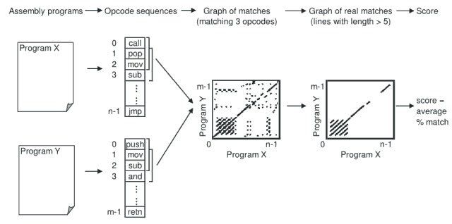
Figure 2: Computing Similarity
We analyzed 45 viruses generated by four virus generators obtained from VX Heavens [29]. We also compared randomly-chosen utility programs from Cygwin [7] to see how viruses differ from these "normal" executable files. These 45 programs consisted of:
The virus variants were named after their generators as follows:
The viruses created by the virus generators consist of assembly code. To provide for more realistic testing, we employed the following procedure. First, virus executable files were created by assembling the viruses using the Borland Turbo Assembler TASM 5.0. Then the generated executables were disassembled using the IDA Pro Disassembler version 4.6.0 [3]. All of the disassembling used the same default settings. The Cygwin utilities were also disassembled by IDA Pro.
We added the prefix "IDA_" to the respective file names to denote that the files were disassembled ASM files created by IDA Pro. For example, the file disassembled from R0.EXE was named IDA_R0.ASM.
We compared the disassembled ASM files instead of the original assembly code generated by the virus generators. We believed by assembling and disassembling with the same tools using the same settings, we have provided a more realistic test environment. That is, this standardized disassembling process is necessary since, in practice, we would start with executable files. In this way, our similarity scores better reflect the effectiveness of the metamorphism as observed in "the wild".
We compared each test virus to all other test viruses produced by the same generator. The resulting similarity scores give us a way to determine how effective each generator is at creating metamorphic variants. For each pair of virus variants under consideration, we computed the similarity score using the method described above in Section 4.1. Comparisons were also made between the normal (Cygwin) files. The raw similarity scores of all the comparisons are given in Table A-1 through Table A-5 in Appendix A of [31]. Figure 3 below is a scatter plot showing the similarity scores for the 190 pair-wise comparisons between the 20 NGVCK viruses and the 190 pairwise comparisons between the 20 normal files. Clearly, similarities between NGVCK virus variants are significantly lower than those between normal files. The minimum, maximum, and average scores of each generator and the normal files are summarized in Table 1.
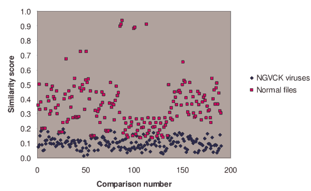
Figure 3: NGVCK Similarity
| Minimum, maximum, and average similarity scores | |||||
|---|---|---|---|---|---|
| NGVCK | G2 | VCL32 | MPCGEN | Normal | |
| min | 0.01493 | 0.62845 | 0.34376 | 0.44964 | 0.13603 |
| max | 0.21018 | 0.84864 | 0.92907 | 0.96568 | 0.93395 |
| average | 0.10087 | 0.74491 | 0.60631 | 0.62704 | 0.34689 |
NGVCK generates viruses with similarities ranging from 1.5% to 21.0% with an average of about 10.0%. This is a far lower degree of similarity than any of the other three generators. For the non-NGVCK generators, the similarity between two variants of the same virus range from 34.4% to 96.6%, and the average scores of G2, VCL32, and MPCGEN are 74.5%, 60.6%, and 62.7%, respectively. On the other hand, normal files give an average similarity of 34.7%. From these results, we can see that the NGVCK viruses are substantially different from one another, while the virus variants generated by the other generators are more similar to one another than normal files. We conclude that the non-NGVCK generators we tested are not nearly as effective as NGVCK at generating metamorphic viruses.
Our similarity results are represented graphically by the bubble graph in Figure 4. Here the minimum score is shown along the x-axis, the maximum score is shown along the y-axis, and the size of the bubble represents the average similarity. Under this representation, an effective generator would have a bubble that is close to the origin and also has a small size.
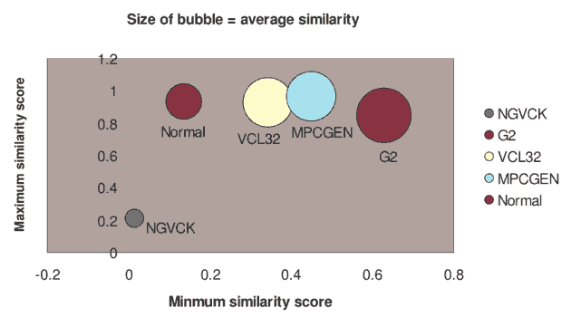
Figure 4: Bubble Graph
As can be seen in Figure 4, NGVCK clearly outperforms the other generators in terms of generating different-looking viruses. VCL32 and MPCGEN have similar morphing ability as their variants have comparable minimum, maximum, and average similarities. G2 viruses have a higher average similarity, as is represented by the bigger bubble size, although the maximum similarity of the variants is lower than that of VCL32 and MPCGEN viruses. Normal files have similarities higher than NGVCK viruses but lower than virus variants produced by the other three generators.
Figures 5 through 9 show the similarity graphs of selected virus pairs. For each generator, we chose a representative pair which has a similarity close to the average similarity score. The first column gives the virus names with the similarity score in parenthesis. The second column shows the graph of all matches, as discussed in Section 4.1, above. The third column shows the graph of matches after noise and random matches have been removed (also discussed in Section 4.1, above).
If we take a closer look at the graphs for the pair of G2 viruses (Figure 6) and the pair of VCL32 viruses (Figure 7), we can see that the matching opcodes are almost all along the diagonal. This indicates that these virus variants have identical opcodes at identical positions, which is obviously not effective metamorphism. On the other hand, the matches between the MPCGEN virus pair are off the diagonal, which shows that identical opcodes appear in different positions of the two virus variants. From this evidence, we can say that MPCGEN has a somewhat greater morphing ability than either G2 or VCL32. However, NGVCK is the most effective since the matching segments are very short and matches are off of the diagonal. Even if we consider the NGVCK pair with the highest similarity (IDA_NGVCK7 and IDA_NGVCK14, with similarity of 21.0%), the match segments are short and off the diagonal. The similarity graph for this pair appears in Figure 10.
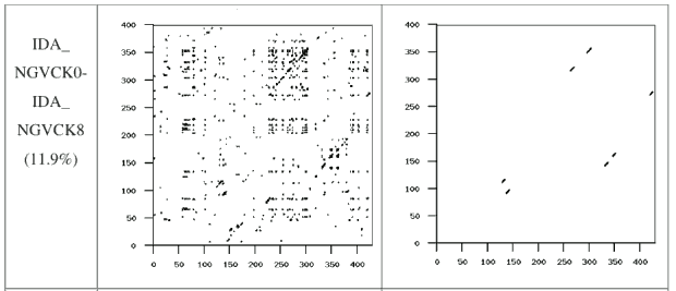
Figure 5: Typical NGVCK Similarity Graph
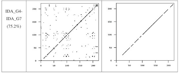
Figure 6: Typical G2 Similarity Graph
Since NGVCK was found to be the most effective metamorphic engine in our test set, we were interested to know how the viruses it produces differ from the viruses created using the other generators. We compared the first 10 NGVCK viruses (IDA_NGVCK0 to IDA_NGVCK9) against each of the following viruses:
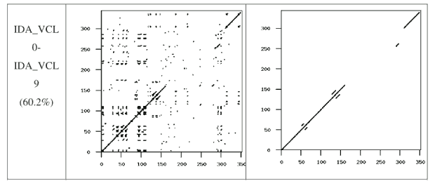
Figure 7: Typical VCL32 Similarity Graph
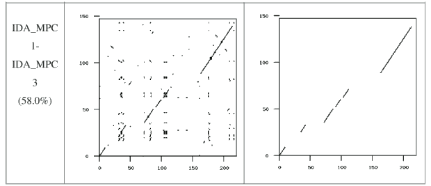
Figure 8: Typical MPCGEN Similarity Graph
Our results show that the NGVCK viruses are very different from the other viruses. Each of the comparisons against the G2 viruses and against the MPCGEN viruses produces a similarity score of zero. Of the 100 comparisons against the VCL32 viruses, 57 comparisons yield a similarity score of zero, while the 43 comparisons that have nonzero similarity have scores range from 1.2% to 5.5%, with an average of just 2.4%. These scores are very low compared to the similarity scores discussed above. The scores for the 43 pairs that have similarity greater than zero appear here in Table A-6 in Appendix A of [31]. The similarity graphs of the pair IDA_NGVCK0 and IDA_VCL4, which has the highest similarity score of such pairs (at 5.5%), is shown in Figure 11.
We also compared the NGVCK viruses to the normal files. All 20 NGVCK viruses were compared to the 20 normal files. All but eight of these 400 comparisons show no similarity. The eight pairs that show some similarity have low scores - in the range of 0.98% to 1.12%. These scores appear below in Table 2.
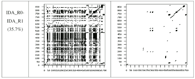
Figure 9: Typical Normal (Cygwin) Similarity Graph
| Similarity scores between files: | |||||||||
|---|---|---|---|---|---|---|---|---|---|
| IDA_NGVCK2 | IDA_R11 | 0.01001 |
| ||||||
| IDA_NGVCK5 | IDA_R10 | 0.01123 | |||||||
| IDA_NGVCK6 | IDA_R16 | 0.01021 | |||||||
| IDA_NGVCK7 | IDA_R5 | 0.0.1007 | |||||||
| IDA_NGVCK7 | IDA_R6 | 0.00981 | |||||||
| IDA_NGVCK7 | IDA_R7 | 0.00990 | |||||||
| IDA_NGVCK7 | IDA_R8 | 0.01010 | |||||||
| IDA_NGVCK7 | IDA_R13 | 0.01115 | |||||||
Table 2: Nonzero NGVCK Similarity
The NGVCK comparison results are displayed using bubble graphs in Figure 12. The bubble labeled "NGVCK vs NGVCK" summarizes the results obtained by comparing NGVCK viruses to NGVCK viruses. This graph illustrates that NGVCK viruses not only have low similarities in comparison to other NGVCK variants, they exhibit even lower similarities when compared to other viruses or normal programs. We conclude that NGVCK viruses are not only highly metamorphic, but that they are also very different from the other viruses in our test set and from the non-viral programs tested.
Since the NGVCK viruses are highly metamorphic, we would expect that they are more difficult to detect than the other metamorphic viruses we tested. Next, we develop a detection method based on hidden Markov models and we also consider detection using a straightforward similarity index calculation. Finally, we test three commercial virus scanners to determine how effective they are at detecting the viruses in our test set.
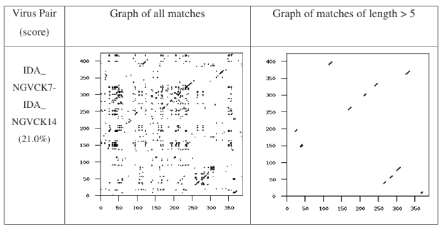
Figure 10: NGVCK Maximum Similarity Graph
In this section, we consider using hidden Markov models (HMMs) to detect metamorphic virus variants. In particular, we want to determine whether HMMs can effectively detect highly metamorphic viruses, such as NGVCK.
In an HMM, we assume there is a Markov process which we cannot directly observe, that is, the Markov process is hidden. We are able to indirectly obtain information about the Markov process from an observation sequence, where each observation is related to the underlying Markov process by a probability distribution.
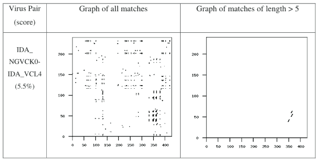
Figure 11: Similarity of NGVCK with VCL32
To fix the notation, let
 = the length of the observed sequence
 = the number of states in the model
 = the number of distinct observation symbols
 = the observation sequence =
 = the sequence of states of the Markov process =
 = the set of observation symbols =
 matrix of the state transition p robability distributions
 matrix of the observation probability distributions
 matrix containing the initial state distribution
 = the HMM model.
Note that the observation symbols are associated with the  . This is not necessary, but it does simplify the notation. Also, since the matrices
  and
and  contain probability distributions, these matrices are row-stochastic. The relationship between
  , and
, and  is illustrated in Figure 13, where the area above the dotted line represents the hidden part of the model.
The following three problems can be solved efficiently using hidden Markov models:
 and a sequence of observations
  , find
  . Here, we want to determine the likelihood of the observed sequence
  , given the model.
 and an observation sequence
  , find an optimal state sequence for the underlying Markov process. In other words, we can uncover the hidden part of the HMM.
 and
and  and
and  (which determine the dimensions of the matrices
  and
and  ), find the model
  that maximizes the probability of observing
  . This can be viewed as training the model to best fit the observed data. Equivalently, we can view this as a (discrete) hill climb on the parameter space represented by
  and
and  .
.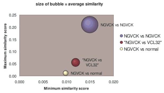
Figure 12: Metamorphic Similarity Scores
![Figure 13: Hidden Markov Model [23]](img/aww00/figd.gif)
Figure 13: Hidden Markov Model [23]
It is, perhaps, not surprising that these three problems can be solved. However, the practical utility of hidden Markov models arises from the fact that efficient algorithms exist to solve each of these problems. We will not discuss the algorithmic details here; for more information, see [23] or [18].
Given a sufficiently long sequence of observations, we can train a model, that is, we can determine the  and
and  matrices in Figure 13, by solving Problem 3, above.
These matrices will be optimal in the sense that they maximize the expected number of states that are correct. Given a trained model, and a sequence of observations, by solving Problem 1, we obtain a score for the sequence, which measures how well it fits the derived model. In this paper, we will not consider Problem 2 further, but we note in passing that a solution to this problem can provide insight into the underlying Markov process, which, in turn, might lead to an improved model.
One useful feature of HMMs is that the a priori assumptions are minimal. Additional strengths of an HMM approach include simplicity and efficiency.
Consider the following application of HMMs. Suppose that we are given a large quantity of written English text, and we remove all punctuation, symbols and numbers, and we convert all letters to lower case. Then we are left with a long sequence of observations consisting of 27 symbols - the 26 lower-case letters and the word space. Now suppose that we train an HMM on this sequence of observation, using  hidden states. That is, we assume that there exists a Markov process, with a
  state transition matrix
  , that generates the observed sequence of states. These states are hidden, but we assume that the sequence of letters that we observe are generated based on these hidden states and the probability distributions in the
  matrix
  . The matrix
  is row stochastic, since row
  is the probability distribution on the observation symbols when the (hidden) Markov process is in state
  .
.
Using the given observation sequence, we can train the HMM, that is, we determine the model  that best fits the observations. The resulting model can then be used to score an unknown sequence of letters (and spaces) to determine whether it corresponds to English text or not. Note that this approach will detect English text that has been "disguised" by a transformation such as a simple substitution cipher.
We tested this English text experiment, using as our set of observations the first T = 50, 000 letters (converted to lower case, with punctuation and special symbols removed) from the "Brown Corpus" of English [5]. We initialized each element of  and
and  randomly to approximately 1/2, with the row-stochasitic condition enforced. The precise initial values used in this example were
![\pi=[0.51316\ 0.48684]](../img/cache/9cbc1801bbf58f480834311a0b564558.gif)
and
![A=\left[0.47468\ 0.52532\\0.51656\ 0.48344\right]](../img/cache/2f210d1dc975415779df2393bc3a1584.gif) .
.Each element of  was initialized to approximately 1/27, ensuring that the probabilities in each row sum to one.1 The precise values in the rows of the initial
  matrix appear in the second and third columns of Table 3, respectively.
| symbol | Initial | Final |
|---|---|---|
| a | 0.03735 0.03909 | 0.13845 0.00075 |
| b | 0.03408 0.03537 | 0.00000 0.02311 |
| c | 0.03455 0.03537 | 0.00062 0.05614 |
| d | 0.03828 0.03909 | 0.00000 0.06937 |
| e | 0.03782 0.03583 | 0.21404 0.00000 |
| f | 0.03922 0.03630 | 0.00000 0.03559 |
| g | 0.03688 0.04048 | 0.00081 0.02724 |
| h | 0.03408 0.03537 | 0.00066 0.07278 |
| i | 0.03875 0.03816 | 0.12275 0.00000 |
| j | 0.04062 0.03909 | 0.00000 0.00365 |
| k | 0.03735 0.03490 | 0.00182 0.00703 |
| l | 0.03968 0.03723 | 0.00049 0.07231 |
| m | 0.03548 0.03537 | 0.00000 0.03889 |
| n | 0.03735 0.03909 | 0.00000 0.11461 |
| o | 0.04062 0.03397 | 0.13156 0.00000 |
| p | 0.03595 0.03397 | 0.00040 0.03674 |
| q | 0.03641 0.03816 | 0.00000 0.00153 |
| r | 0.03408 0.03676 | 0.00000 0.10225 |
| s | 0.04062 0.04048 | 0.00000 0.11042 |
| t | 0.03548 0.03443 | 0.01102 0.14392 |
| u | 0.03922 0.03537 | 0.04508 0.00000 |
| v | 0.04062 0.03955 | 0.00000 0.01621 |
| w | 0.03455 0.03816 | 0.00000 0.02303 |
| x | 0.03595 0.03723 | 0.00000 0.00447 |
| y | 0.03408 0.03769 | 0.00019 0.02587 |
| z | 0.03408 0.03955 | 0.00000 0.00110 |
| space | 0.03688 0.03397 | 0.33211 0.01298 |
Table 3: Initial and Final B
Using these initial values, we solved HMM Problem 3 (discussed above), that is, we determine the model that best fits the observations. The solution to Problem 3 is an iterative process and after the initial iteration, we find
![\log[P(O|\lambda)]=-165097.29](../img/cache/758512b3c08a79917f5dec33a9f3a7a4.gif)
and after 100 iterations,
![\log[P(O|\lambda)]=-137305.28.](../img/cache/01d7eb04c425334cc217837a7ed21651.gif)
This indicates that the "score" for the model has improved significantly. In fact, after 100 iterations, the model  has converged to
![\pi=[0.00000\ 1.00000]](../img/cache/553971f78a981a718815b9bd36bc6f49.gif)
and
![A=\left[0.25596\ 0.74404\\0.71571\ 0.28429\right]](../img/cache/24e9178dc7689a0a9cd549ae72f3de2d.gif)
with the converged rows of  appearing in the last two columns of Table 3.
The converged  matrix is particularly interesting. Without having made any a priori assumption about the two hidden states, the
  matrix indicates that one hidden state corresponds to vowels while the other hidden state corresponds to consonants. Curiously, word-space is more "vowel-like", while the letter "y" is almost never a vowel. Of course, anyone familiar with English would not be too surprised that there is a clear distinction between vowels and consonants. But the HMM result show us that this distinction is a statistically significant feature inherent in the language. And, thanks to HMMs, the vowel-consonant split could easily be deduced by anyone armed with HMMs - even someone who has no background knowledge of the English language.
Cave and Neuwirth [6] obtain further interesting results for this English text example by considering cases with more than two hidden states. They are able to sensibly interpret the results for models having up to 12 hidden states.
Given a set of metamorphic virus variants, we propose to train a hidden Markov model. The resulting model can be viewed as representing the statistical properties of the virus family. The trained model can then be used to determine the probability that a given program belongs to the same virus family as the training set.
We trained our models using the assembly opcode sequences of the metamorphic virus files. We first pre-processed the viruses following the same procedure used in the similarity tests discussed in Section 4. That is, we disassembled the executable files and extracted sequences of opcodes from each. For training, we simply concatenated the opcode sequences to yield one long observation sequence. Note that the HMM process we follow here is analogous to the English text example discussed above.
When trained with multiple sequences, the resulting HMM represents the "average" behavior of all of the sequences in the form of a statistical profile. In this way, we can represent an entire virus family with a single HMM.
After training a model, we used the resulting HMM to compute the log likelihood for each virus variant in the test set and also for each program in the comparison set. Here, the test set consists of viruses in the same family as those used for training, while the comparison set includes normal (non-viral) programs and viruses in other families. Since the log likelihood is length dependent, we normalized the score by dividing by the length to obtain the log likelihood per opcode (LLPO). This LLPO score is length independent.
Comparing the scores of the files in the test set with the scores of files in the comparison set, we hope to see a clear separation between the two sets. More precisely, the trained model should assign higher LLPO scores to files belonging to the virus family used to train the model. From these empirical scores, we can determine a threshold, above which we will classify a file as belonging to the same family as the viruses in the training set.
Our data set consisted of 200 viruses generated by the Next Generation Virus Creation Kit (NGVCK), which was shown to have the most effective metamorphism of the virus generators tested in Section 4. With five-fold cross validation, the number of viruses in each test set was 40 and the number of sequences used for training was 160 for each model.
Each virus in our training set consisted of about 350 to 450 opcodes, with an average length of 416. Concatenating 160 viruses to train a model resulted in an observation training sequence of length 66,650, on average, with the precise length depending on the particular set of viruses selected for training. We tested several HMM models, where  , the number of hidden states, ranged from two to six. The number of distinct opcodes in the observation sequence determined
  , the number of possible observations. In our experiments,
  ranged from 70 to 80.
After training, we computed the scores of the 40 family viruses in the test set to determine a threshold. Then we tested the model against a set of 65 files consisting of both benign and viral programs. These included:
The files were processed as described in Section 4, above. In particular, the executable files were disassembled using IDA Pro [11].
Our purpose here is to determine how well the HMM can separate viruses in the test set from the benign programs and viruses in other families. We refer to the viruses in the test set as "family viruses", since they were generated by the same virus generator (NGVCK) as that used for training. This is in contrast to the "non-family viruses" in the comparison set, which were produced by other metamorphic virus generators. The random utility files in the comparison set are the "normal files".
The results in Figure 14 are typical. From these results it is clear that we can set a threshold whereby the family viruses are always distinguished from the normal files - see [31] for more details on thresholding. There are some false positives, but these are entirely due to non-family viruses, so it is not unreasonable to consider these misclassifications as a beneficial feature - rather than a flaw - in this virus detection technique.
As discussed in the English text example, above, one interesting aspect of HMMs is that we can sometimes use the trained model to gain insight into the underlying (hidden) Markov process. An example of a converged  matrix - for an HMM trained on NGVCK viruses - appears in Table 4. Note that in this example, the number of hidden state is
  , the number of observation symbols is
  , and
, and  observation were used to train the model. See [31] for more examples of such matrices and further discussion.
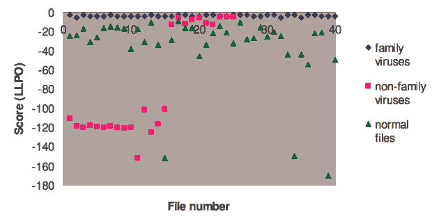
Figure 14: LLPO Scores
In the similarity tests described in Section 4, we found that viruses generated by the Next Generation Virus Creation Kit (NGVCK) are, on average, only about 10% similar to each other. They share even lower similarities when compared to normal programs (0 to 1.1%), and when compared to other viruses not in the same family (0 to 5.5%). Since these NGVCK viruses are so different from other programs - benign or viral - it is possible to distinguish them by using only the similarity index.
This similarity-based detection method works as follows. To classify whether a program belongs to the NGVCK virus family, compare the program to any randomly chosen NGVCK virus. If it has no similarity to the NGVCK virus, it is classified as non-family (i.e., not belonging to the NGVCK family). Otherwise, we compare several more NGVCK viruses to the chosen NGVCK virus to determine a threshold. If the similarity score of the program with the original chosen NGVCK virus is higher than the threshold value, it is classified as a family virus.
We used this approach to classify the 40 family viruses IDA_N0 through IDA_N39, the 40 normal files, and the 25 non-family viruses used in the tests in Section 4 (for a total of 105 viruses). We conducted two tests where we compared these files to IDA_N146 and IDA_N101, respectively. The similarity scores for the test involving IDA_N146 appear in Table 5.
The column on the right in Table 5 shows the minimum and the maximum score when IDA_N146 was compared to other NGVCK viruses. Simply using the minimum score of 0.0349 as the threshold, we were able to correctly classify all 105 files tested.
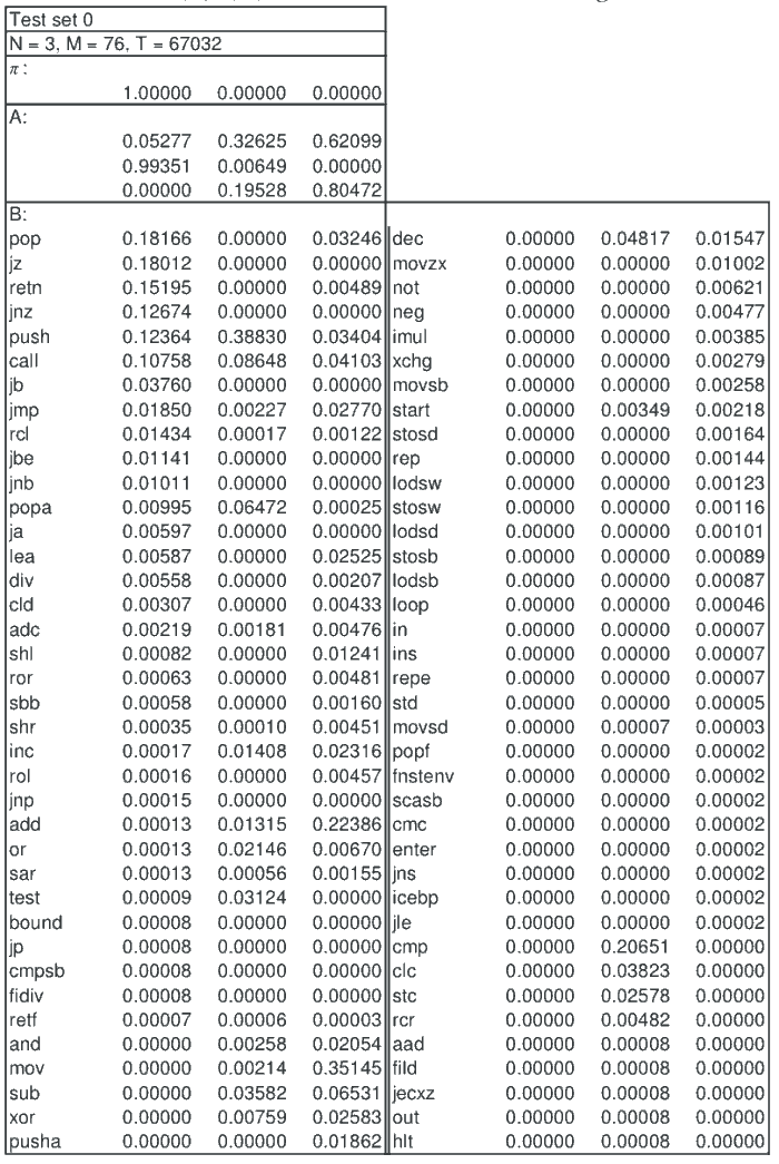
Table 4: Converged B Matrix
All family viruses had scores greater than 0.0349 while all other programs scored lower than the threshold value. In other words, the detection rate was 100% and the false positive rate was 0% in this test.
The test using IDA_N101 also achieved a 100% detection rate and a 0% false positive rate. This straightforward approach, which uses the similarity index for classification, worked remarkably well in our two tests - the accuracy was 100% and there were no false positives or false negatives in either case.
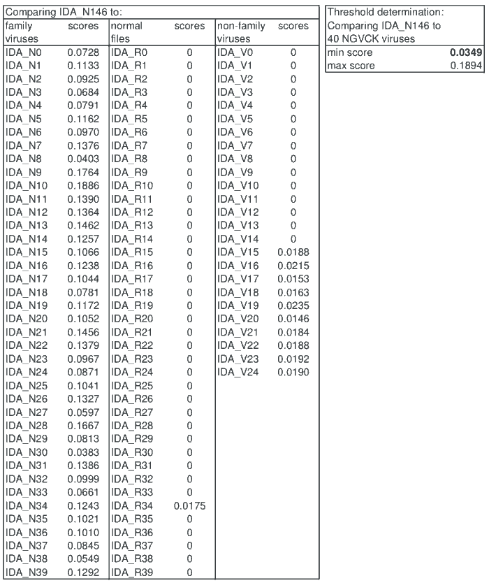
Table 5: Similarity Scores
In this section we consider the effectiveness of commercial scanners in detecting the metamorphic viruses in our test set. We stored 37 virus executables in a folder and scanned the folder using each of the following scanners:
The 37 viruses we tested were all used in our HMM tests in Section 4. Specifically, these executables included:
We found that eTrust and avast! each detected 17 viruses. Both of these scanners detected the G2 viruses and the MPCGEN viruses, but not those generated by VCL32 or NGVCK. The AVG Anti-Virus scanner detected 27 viruses, namely, all of the G2, MPCGEN and VCL32 viruses. The 10 NGVCK viruses were not detected by any of these three scanners.
The eTrust detector relies on signature detection, and it identified the G2 viruses as belonging to the Anarchy family while the MPCGEN viruses were correctly classified as the PS-MPC family. Avast! antivirus classified all MPCGEN virus infections as PS/MPC-gen and all G2 virus infections as PS/G2-B [31].
Of the seven MPCGEN viruses, AVG classified three as "could be infected PS-MPC" while the other four MPCGEN viruses and nine of the G2 viruses were classified as unknown viruses. The scanner misclassified all VCL32 viruses as Win32/Ngvck.W, while none of the NGVCK viruses were actually detected [31].
NGVCK viruses were able to evade detection by all three commercial scanners that we tested. However, as discussed above, both the similarity index approach and the hidden Markov model approach were able to identify the NGVCK viruses with high accuracy. We conclude that HMM and similarity-based scanning are effective methods for detecting the highly metamorphic NGVCK viruses.
Virus writers and anti-virus researchers generally agree that metamorphism is a potent method for generating difficult-to-detect viruses. Several virus writers have released virus creation kits and claimed that they possess the ability to automatically produce morphed virus variants that look substantially different from one another.
We measured the similarity between virus variants generated by four virus generators downloaded from the Internet. Our results show that the effectiveness of these generators varies widely. While the best generator, NGVCK, is able to create viruses that share only a few percent of similarity, the other generators produce viruses that are over 60% similar, on average. Randomly-selected utility files have a similarity of about 35%, which indicates that, with the exception of NGVCK, the virus creation kits we tested do not effectively morph the viral code.
Clearly, the NGVCK viruses have the highest degree of metamorphism among the four virus families we tested. In addition, NGVCK viruses are very different from normal programs and viruses in other families.
To detect metamorphic virus variants, we experimented with hidden Markov models (HMMs). Using HMMs, we can distinguish NGVCK viruses from normal programs. If the variants of a metamorphic virus are sufficiently different that signature-based scanning cannot detect a newly morphed variant, the HMM approach may provide a feasible means of detection.
The fact that NGVCK viruses have assembly code structure that is so different from normal programs and other viruses makes them detectable by a similarity index approach as well. This result tends to indicate that even though the NGVCK viruses show a high degree of metamorphism, they are "too different" from normal programs, making them susceptible to similarity-based detection. The similarity index approach is surprisingly effective when the virus code structure is significantly different from non-viral code.
We scanned the test viruses from the four metamorphic families using three commercial virus scanners. All non-NGVCK viruses were detected by the scanners, while all NGVCK viruses escaped detection by these scanners. While the NGVCK viruses were not detected by the scanners we tested, we have shown that both the similarity index approach and the HMM approach are effective in dealing with these viruses.
To avoid detection, it appears that metamorphic viruses require not only a high degree of metamorphism, but also a degree of similarity to normal programs. None of the virus construction kits we tested satisfy both of these requirements. Of course, we cannot rule out the possibility that metamorphic viruses can be constructed that satisfy both of these conditions. However, it appears to be a non-trivial challenge to construct such viruses.
It is interesting to contrast the use of metamorphism in virus construction with the case where metamorphism is used for defense, as discussed in Section 2.3. To prevent buffer overflow attacks, for example, a small degree of metamorphism is highly effective, while it appears to be challenging for malware writers to gain a significant advantage from metamorphic software. That is, the results resented in this paper, together with [10], provide evidence that metamorphic software is inherently more advantageous when used for good rather than evil. As a general rule in information security, the inherent advantage tends to lie with the attackers [25]. Perhaps metamorphic software is one of the exceptions to this rule.
1 If  and
and  are set to uniform probabilities, then the model is at a fixed point and it cannot climb to a solution. Consequently, it is necessary to slightly randomize the initial values.